Getting Started on Geospatial Analysis with Python, GeoJSON and GeoPandas
Time to read: 6 minutes
August 14, 2017
Written by

As a native New Yorker, I would be a mess without Google Maps every single time I go anywhere outside the city. We take products like Google Maps for granted, but they’re an important convenience. Products like Google or Apple Maps are built on foundations of geospatial technology. At the center of these technologies are locations, their interactions and roles in a greater ecosystem of location services.
This field is referred to as geospatial analysis. Geospatial analysis applies statistical analysis to data that has geographical or geometrical components. In this tutorial, we’ll use Python to learn the basics of acquiring geospatial data, handling it, and visualizing it. More specifically, we’ll do some interactive visualizations of the United States!
Environment Setup
This guide was written in Python 3.6. If you haven’t already, download Python and Pip. Next, you’ll need to install several packages that we’ll use throughout this tutorial. You can do this by opening terminal or command prompt on your operating system:
Since we’ll be working with Python interactively, using the Jupyter Notebook is the best way to get the most out of this tutorial. Following this installation guide, once you have your notebook up and running, go ahead and download all the data for this post here. Make sure you have the data in the same directory as your notebook and then we’re good to go!
A Quick Note on Jupyter
For those of you who are unfamiliar with Jupyter notebooks, I’ve provided a brief review of which functions will be particularly useful to move along with this tutorial.
In the image below, you’ll see three buttons labeled 1-3 that will be important for you to get a grasp of: the save button (1), add cell button (2), and run cell button (3).
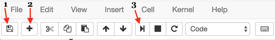
The first button is the button you’ll use to save your work as you go along (1). Feel free to choose when to save your work.
Next, we have the “add cell” button (2). Cells are blocks of code that you can run together. These are the building blocks of jupyter notebook because it provides the option of running code incrementally without having to to run all your code at once. Throughout this tutorial, you’ll see lines of code blocked off. Each line of code should correspond to a cell.
Lastly, there’s the “run cell” button (3). Jupyter Notebook doesn’t automatically run it your code for you; you have to tell it when by clicking this button. As with add button, once you’ve written each block of code in this tutorial onto your cell, you should then run it to see the output (if any). If any output is expected, note that it will also be shown in this tutorial so you know what to expect. Make sure to run your code as you go along because many blocks of code in this tutorial rely on previous cells.
Introduction
Data typically comes in the form of a few fundamental data types: strings, floats, integers, and booleans. Geospatial data, however, uses a different set of data types for its analyses. Using the shapely module, we’ll review what these different data types look like.
shapely has a class called geometry that contains different geometric objects. Using this module we’ll import the needed data types:
The simplest data type in geospatial analysis is the Point data type. Points are objects representing a single location in a two-dimensional space, or simply put, XY coordinates. In Python, we use the point class with x and y as parameters to create a point object:
Notice that when we print p1, the output is POINT (0 0). This indicated that the object returned isn’t a built-in data type we’ll see in Python. We can check this by asking Python to interpret whether or not the point is equivalent to the tuple (0, 0):
The above code returns False because of its type. If we print the type of p1, we get a shapely Point object:
Next we have a Polygon, which is a two-dimensional surface that’s stored as a sequence of points that define the exterior. Because a polygon is composed of multiple points, the shapely polygon object takes a list of tuples as a parameter.
Oddly enough, the shapely Polygon object will not take a list of shapely points as a parameter. If we incorrectly input a Point, we’ll get an error message remind us of the lack of support for this data type.
Data Structures
GeoJSON is a format for representing geographic objects. It’s different from regular JSON because it supports geometry types, such as: Point, LineString, Polygon, MultiPoint, MultiLineString, MultiPolygon, and GeometryCollection.
Using GeoJSON, making visualizations becomes suddenly easier, as you’ll see in a later section. This is primarily because GeoJSON allows us to store collections of geometric data types in one central structure.
GeoPandas is a Python module used to make working with geospatial data in python easier by extending the datatypes used by the Python module pandas to allow spatial operations on geometric types. If you’re unfamiliar with pandas, check out these tutorials here.
Typically, GeoPandas is abbreviated with gpd and is used to read GeoJSON data into a DataFrame. Below you can see that we’ve printed out five rows of a GeoJSON DataFrame:
Just as with regular JSON and pandas dataframes, GeoJSON and GeoPandas have functions which allow you to easily convert one to the other. Using the example dataset from above, we can convert the DataFrame to a geojson object using the to_json function:
Being able to easily convert GeoJSON from one format to another gives us more freedom as to what we can do with our data, whether that be analyzing, visualizing, or manipulating.
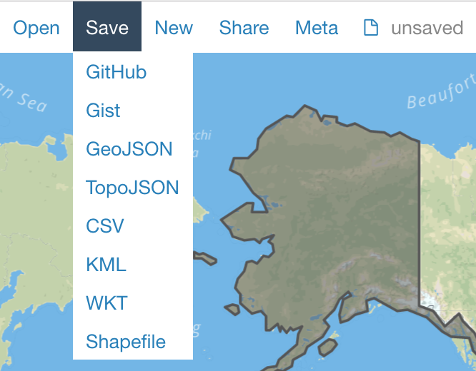
Next we will review geojsonio, a tool used for visualizing GeoJSON on the browser. Using the states dataset above, we’ll visualize the United States as a series of Polygons with geojsonio’s display function:
Once this code is run, a link will open in the browser, displaying an interface as shown below:
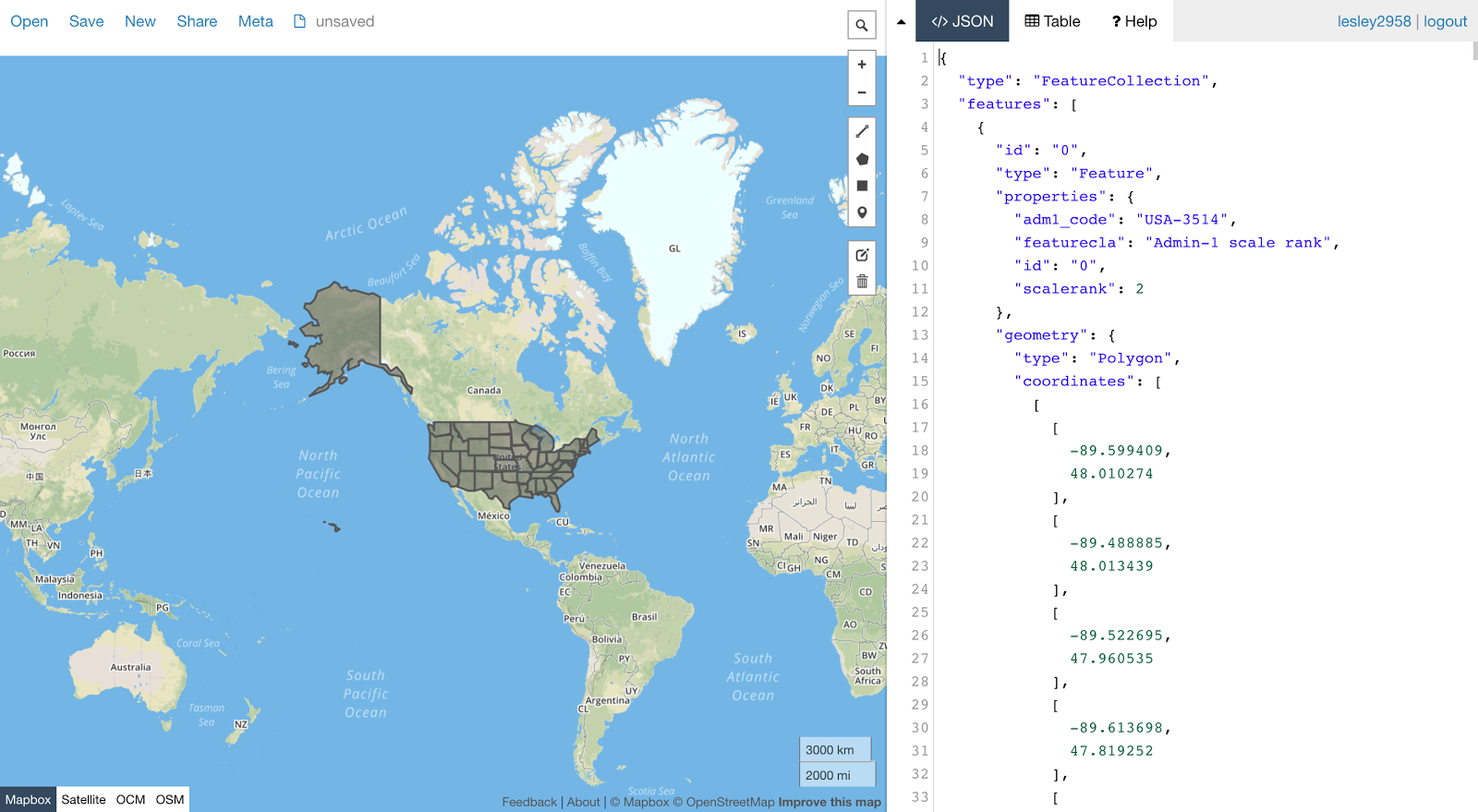
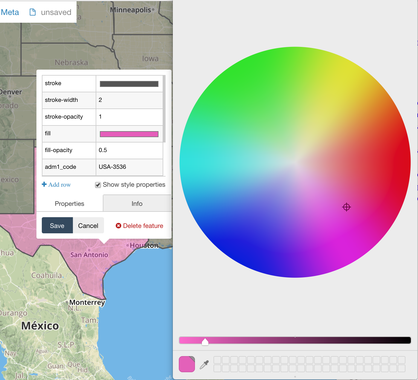
On the left of the page, you can see that the GeoJSON displayed and available for editing. If you zoom in and select a geometric object, you’ll see that you also have the option to customize it:
And perhaps most importantly, geojsonio has multiple options for sharing your content. There is the option to share a link directly:
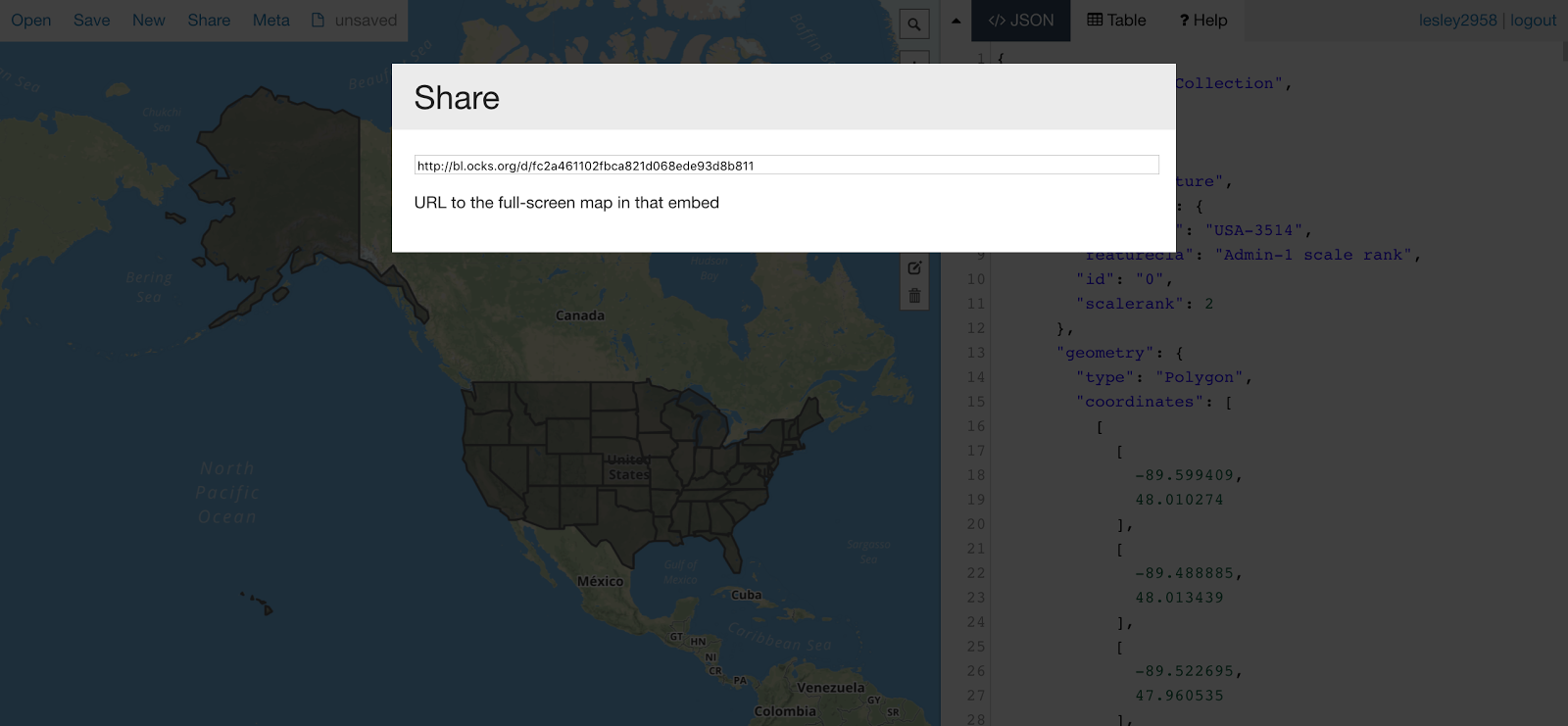
And to everyone’s convenience the option to save to GitHub, GitHub Gist, GeoJSON, CSVs, and various other formats gives developers plenty of flexibility when deciding how to share or host content.
In the example before we used GeoPandas to pass GeoJSON to the display function. If no manipulation on the geospatial needs to be performed, we can treat the file as any other and set its contents to a variable:
The format is still a suitable parameter for the display function because JSON is technically a string. Again, the main difference between using GeoPandas is whether or not any manipulation needs to be done.
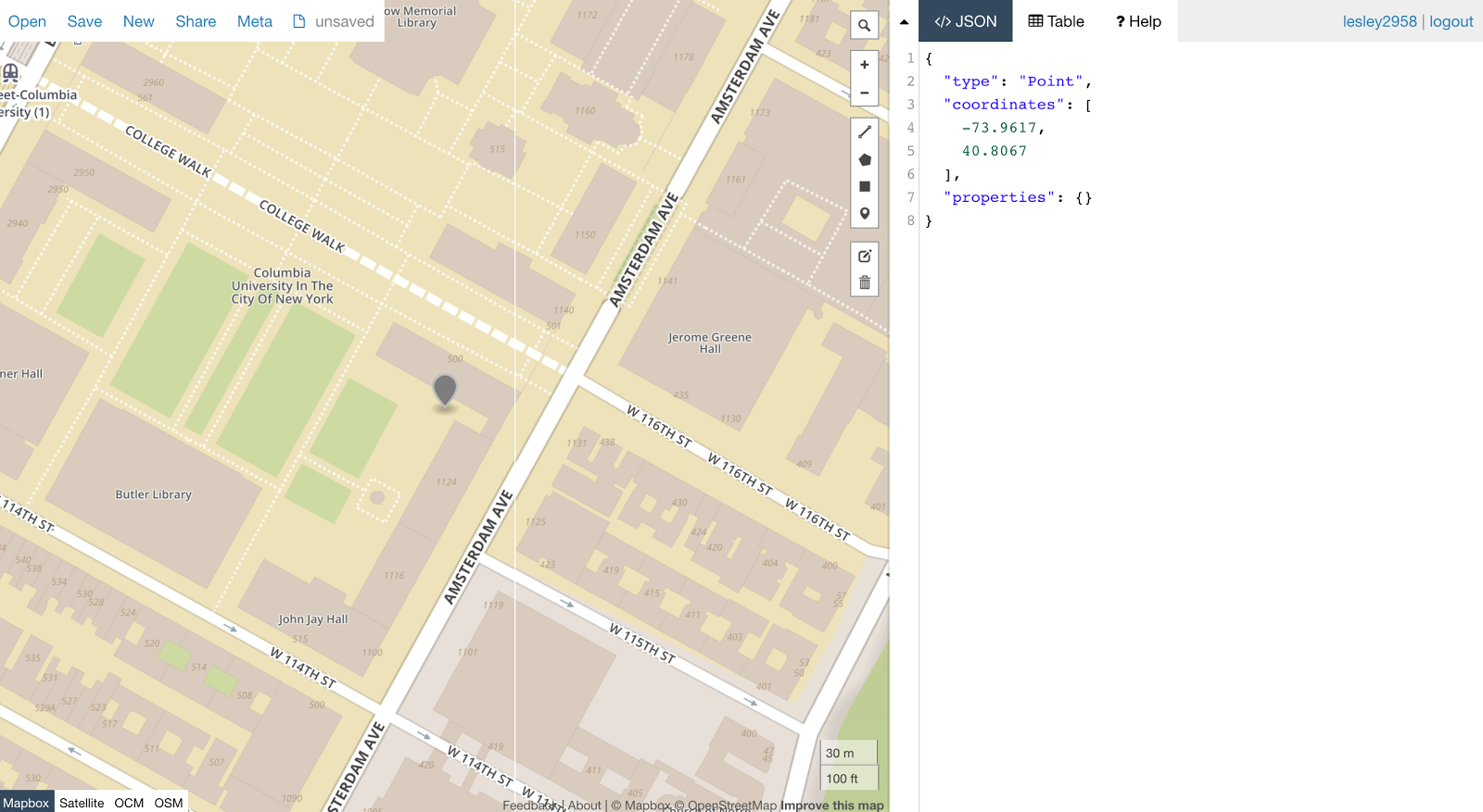
This example is simply a point, so besides reading in the JSON, nothing necessarily has to be done, so we’ll just pass in the GeoJSON string directly:
And once again, a link is opened in the browser and we have this beautiful visualization of a location in Manhattan.
And That’s a Wrap
That wraps up an introduction to performing geoSpatial analysis with Python. Most of these techniques are interchangeable in R, but Python is one of the best suitable languages for geospatial analysis. Its modules and tools are built with developers in mind, making the transition into geospatial analysis must easier.
In this tutorial, we visualized a map of the United States, as well as plotted a coordinate data point in Manhattan. There are multiple ways in which you can expand on these exercises & state outlines are crucial to so many visualizations created to compare results between states.
Moving forward from this tutorial, not only can you create this sort of visualization, but you can combine the techniques we used to plot coordinates throughout multiple states. To learn more about geospatial analysis, check the resources below:
If you liked what you did here, follow @lesleyclovesyou on Twitter for more content, data science ramblings, and most importantly, retweets of super cute puppies.

Related Resources
Twilio Docs
From APIs to SDKs to sample apps
API reference documentation, SDKs, helper libraries, quickstarts, and tutorials for your language and platform.
Resource Center
The latest ebooks, industry reports, and webinars
Learn from customer engagement experts to improve your own communication.
Ahoy
Twilio's developer community hub
Best practices, code samples, and inspiration to build communications and digital engagement experiences.