Data Science and Linear Algebra Fundamentals with Python, SciPy, & NumPy
Time to read:
June 08, 2018
Written by

Math is relevant to software engineering but it is often overshadowed by all of the exciting tools and technologies. In the field of data science, however, being familiar with linear algebra and statistics is very important to statistical analysis and prediction. In this tutorial, we’ll use SciPy and NumPy to learn some of the fundamentals of linear algebra and statistics.
Getting Started
We’ll be using Python to show how different statistical concepts can be applied computationally. Specifically, we’ll work with NumPy, a scientific computing module for Python.
This guide was written in Python 3.6. If you haven’t already, download Python and Pip. Once you have Python and Pip installed, clone this repo using Git as follows:
The Git repository contains all of the data you’ll need for this tutorial.
Next, install the NumPy, SciPy, and sklearn modules that we’ll use throughout this tutorial:
Since we’ll be working with Python interactively, using a Jupyter Notebook is the best way to get the most out of this tutorial. You already installed it with pip3 up above; now you just need to get it running. Open up your terminal or command prompt and enter the following command:
It should have opened in your default browser. Once it does, we’re ready to go.
For those of you who are unfamiliar with Jupyter Notebooks, I’ve provided a brief review of the functions which will be particularly useful for this tutorial.
In the image below, you’ll see three buttons labeled 1-3 that will be important for you to get a grasp of the save button (1), the add cell button (2), and the run cell button (3).
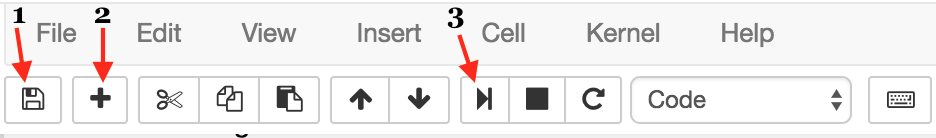
The first button is the button you’ll use to save your work as you go along (1). I won’t give you directions when you should do this — that’s up to you.
Next, we have the “add cell” button (2). Cells are blocks of code that you can run together. These are the building blocks of Jupyter Notebook because it provides the option of running code incrementally without having to run all your code at once. Throughout this tutorial, you’ll see lines of code blocked off — each one should correspond to a cell.
Lastly, there’s the “run cell” button (3). Jupyter Notebook doesn’t automatically run your code for you; you have to tell it when by clicking this button. As with the add button, once you’ve written each block of code in this tutorial onto your cell, you should then run it to see the output (if any). If any output is expected, note that it will also be shown in this tutorial so you know what to expect. Make sure to run your code as you go along because many blocks of code in this tutorial rely on previous cells.
Vectors, Matrices, and NumPy
Because of the nature of data science, we encounter data of all kinds — numerical, text, images, etc. This variety forces us to be creative in the ways we structure our data and led to a need for additional data structures beyond lists and dictionaries, namely, vectors and matrices.
Vectors
Lists are data structures universal to pretty much any programming language. Vectors are very similar to lists, in that a vector is just a set, or collection, of numbers. Because of this similarity, we can represent a vector with a list, for example:
Matrices
A matrix is similar to a list or vector, but there’s one fundamental difference: it’s a 2D array that stores numbers. Another way of thinking about matrices is that they are multiple vectors in an list. Visually, they typically look like:
To access any given element, you would use its row and column number. For example, in the following 3×3 matrix, we would access the number by:
The result provided by Jupyter Notebook should be:
NumPy is a Python module that supports vectors and matrices in an optimized way. Using the built-in data structures of the Python programming language, we just implemented examples of vectors and matrices, but NumPy gives us a better way. Because NumPy is written in C code, it’s also incredibly fast to do:
Here, np.array() and np.matrix() replace the previous techniques we used to represent these data structures.
Math Operations = Data Operations
In the field of data analysis and prediction, operations that produce analyses are typically grounded in mathematical operations, particularly operations in linear algebra. Luckily enough for us, NumPy also supports these functions efficiently.
Within the NumPy module, there are tons of matrix operations you can use; and as with any module, this reduces the amount of code you need to write. In the next section, we’ll review some concrete examples of when these operations occur in the context of a data science-related problem.
Images are Data
Images consist of pixels, which vary in numerical value. But that’s not the important part. The important part is what this structure looks like.
Consider this picture of my very cute dog, Lennon:

This image is 200 x 200 pixels. Does this notation sound familiar to you? It’s how we described the dimensionality of a matrix. Because of this wonderful property, we can literally treat the pixels of an image as an n x n matrix.
In the following example, we’ll do this using SciPy.
Using the imread function to read the image into the img variable gives us a matrix that we can work with. We can verify img is in fact a matrix by printing out its type:
We can manipulate the image so that it’s tinted using a matrix operation.
I arbitrarily chose numbers to do a multiplication operation between the image matrix and this vector.
img_tinted is now a manipulated version of the original photo matrix which we can then save:

As you see above, my dog’s picture looks different—it’s now tinted!
Text is Data
As a bonus, I’ll introduce some beginning steps of a machine learning algorithm for sentiment analysis to see how SciPy plays into this process.
The first natural question is, what is “sentiment analysis”?
Well, it’s exactly what it sounds like: using computational tools to determine the emotional tone behind words.
Sentiment analysis isn’t a new concept. There are thousands of labeled datasets out there, with labels that vary from simple positive and negative to more complex systems that determine how positive or negative a given text is. While it may not be immediately obvious how matrices and vectors fit into this, let’s go ahead and see how this works with tweets.
Converting Tweets to a Matrix
For this post, I’ve selected a dataset consisting of tweets from Twitter already labeled as positive or negative. Using this data, go through the initial steps of building a classifier that predicts whether a tweet is positive or negative. Namely, we’ll set up the data preparation portion of this problem.
It’s important to note that sklearn is a Python module with built-in machine learning algorithms. To utilize these models, having the correct data structures is crucial. Since scikit-learn provides a lot of black box algorithms, it’s much easier to require the same standard data structure — this is where SciPy fits into the picture.
Using sklearn.feature_extraction.text.CountVectorizer, we will convert the tweets to a matrix, or two-dimensional array, of word counts. Ultimately, this data would be used to build the classifier.
First, we import this specific class:
Each file is a text file with one tweet per line. We will use the built-in open() function to split the file line-by-line and build up two lists: one for tweets and one for their labels.
Next, initialize a sklearn vector with the CountVectorizer class. This vectorizer will transform our data into vectors of features.
Notice how we didn’t directly use SciPy? This is because sklearn actually builds the class above with the SciPy module. If you looked at the logs when you installed sklearn, you’ll see that it checks to make sure SciPy installed. This speaks to the importance SciPy plays within machine learning; SciPy provides data structures necessary for machine learning libraries such as scikit-learn.
Just as we converted an image into a matrix that we manipulated, we converted tweets into a matrix which we then transformed to fit our problem. These are just two examples of how data structures local to math, such as vectors and matrices, can be so important in computational problems.
If you liked what you did here, check out my GitHub (@lesley2958) and Twitter (@lesleyclovesyou) for more!
Related Resources
Twilio Docs
From APIs to SDKs to sample apps
API reference documentation, SDKs, helper libraries, quickstarts, and tutorials for your language and platform.
Resource Center
The latest ebooks, industry reports, and webinars
Learn from customer engagement experts to improve your own communication.
Ahoy
Twilio's developer community hub
Best practices, code samples, and inspiration to build communications and digital engagement experiences.