Analyzing Messy Data Sentiment with Python and nltk
Time to read:
September 06, 2017
Written by
This post is part of Twilio’s archive and may contain outdated information. We’re always building something new, so be sure to check out our latest posts for the most up-to-date insights.

Sentiment analysis uses computational tools to determine the emotional tone behind words. This approach can be important because it allows you to gain an understanding of the attitudes, opinions, and emotions of the people in your data.
At a higher level, sentiment analysis involves natural language processing and artificial intelligence by taking the text element, transforming it into a format that a machine can read, and using statistics to determine the actual sentiment.
In this tutorial, we’ll use the natural language processing module, nltk, to determine the sentiment of tweets from Twitter.
Sentiment analysis on text
Sentiment analysis isn’t a new concept. There are thousands of labeled data out there, labels varying from simple positive and negative to more complex systems that determine how positive or negative is a given text. Because there’s so much ambiguity within how textual data is labeled, there’s no one way of building a sentiment analysis classifier.
I’ve selected a pre-labeled set of data consisting of tweets from Twitter already labeled as positive or negative. Using this data, we’ll build a sentiment analysis model with nltk.
Environment Setup
This guide was written in Python 3.6. If you haven’t already, download Python and Pip. Next, you’ll need to install the nltk package that we’ll use throughout this tutorial:
We will use datasets that are already well established and widely used for our textual analysis. To gain access to these datasets, enter the following command into your command line (note that this might take a few minutes):
Using Jupyter Notebook is the best way to get the most out of this tutorial by using its interactive prompts. When you have your notebook up and running, you can download the data we’ll be working with in this example. You can find this in the repo as neg_tweets.txt and pos_tweets.txt. Make sure you have the data in the same directory as your notebook and then we are good to go.
A Quick Note on Jupyter
For those of you who are unfamiliar with Jupyter notebooks, I’ve provided a brief review of which functions will be particularly useful to move along with this tutorial.
In the image below, you’ll see three buttons labeled 1-3 that will be important for you to get a grasp of — the save button (1), add cell button (2), and run cell button (3).
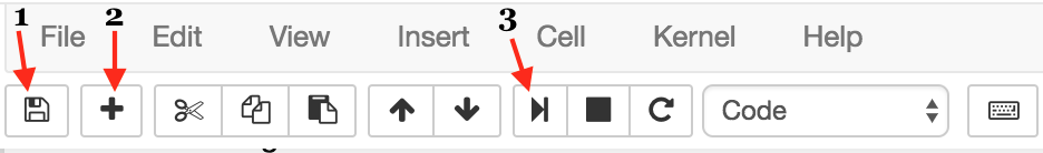
The first button is the button you’ll use to save your work as you go along (1).
Next, we have the “add cell” button (2). Cells are blocks of code that you can run together. These are the building blocks of jupyter notebook because it provides the option of running code incrementally without having to run all your code at once. Throughout this tutorial, you’ll see lines of code blocked off- each one should correspond to a cell.
Lastly, there’s the “run cell” button (3). Jupyter Notebook doesn’t automatically run your code for you; you have to tell it when to do it by clicking “run cell”. As with the add button, once you’ve written each block of code in this tutorial onto your cell, you should then run it to see the output (if any). If any output is expected, note that it will also be shown in this tutorial so you know what to expect. Make sure to run your code as you go along because many blocks of code in this tutorial rely on previous cells.
Preparing the Data
We’ll now use nltk to build a sentiment analysis model on the same dataset. nltk requires a different data format, which is why I’ve implemented the function below:
Which produces
format_sentence changes each tweet into a dictionary of words mapped to True booleans. Though not obvious from this function alone, this will eventually allow us to train our prediction model by splitting the text into its tokens, i.e. tokenizing the text.
Format the positively and negatively labeled data using the data we downloaded from the GitHub repository.
Building a Classifier
All nltk classifiers work with feature structures, which can be simple dictionaries mapping a feature name to a feature value. In this example, we use the Naive Bayes Classifier, which makes predictions based on the word frequencies associated with each label of positive or negative.
SWe can call a function show_most_informative_features to see which words are the highest indicators of a positive or negative label because the Naive Bayes Classifier is based entirely off of the frequencies associated with each label for a given word:
Notice that there are three columns. Column 1 is why we used format_sentence to map each word to a True value. What it does is count the number of occurrences of each word for both labels to compute the ratio between the two, which is what column 3 represents. Column 2 lets us know which label occurs more frequently. The label on the left is the label most associated with the corresponding word.
Classification
Let’s try the classifier out with a positive example to see how our model works:
Outputs:
Now try out an example we’d expect a negative label:
We get the output:
What happens when we mix words of different sentiment labels? Take a look at this example:
Output:
We’ve found a mislabel! Naive Bayes doesn’t consider the relationship between words, which is why it wasn’t able to catch the fact that “no” acted as a negator to the word headache. Instead, it read two negative indicators and classified it as such.
Given that, we can probably expect a less than perfect accuracy rate.
Accuracy
nltk has a built in method that computes the accuracy rate of our model:
The result:
nltk specializes and is made for natural language processing tasks, so we should expect that nltk do fairly well with uncleaned and unnormalized data. But why has this well established models only resulted in ~80% accuracy rates? It goes back to the lack of processing beforehand.
If you look at the actual data, you’ll see that the data is kind of messy – there are typos, abbreviations, grammatical errors of all sorts. There’s no general format to every tweet aside from the fact that each tweet is, well, a tweet. So what can we do about this?
For now, we’re stuck with our 83% accurate classifier.
If you liked what you did here, follow me @lesleyclovesyou on Twitter for more content, data science ramblings, and most importantly, retweets of super cute puppies.


Related Resources
Twilio Docs
From APIs to SDKs to sample apps
API reference documentation, SDKs, helper libraries, quickstarts, and tutorials for your language and platform.
Resource Center
The latest ebooks, industry reports, and webinars
Learn from customer engagement experts to improve your own communication.
Ahoy
Twilio's developer community hub
Best practices, code samples, and inspiration to build communications and digital engagement experiences.