Making Sentiment Analysis Easy With Scikit-Learn

Making Sentiment Analysis Easy With Scikit-Learn

Sentiment analysis uses computational tools to determine the emotional tone behind words. Python has a bunch of handy libraries for statistics and machine learning so in this post we’ll use Scikit-learn to learn how to add sentiment analysis to our applications.

Sentiment Analysis isn’t a new concept. There are thousands of labeled datasets out there, labels varying from simple positive and negative to more complex systems that determine how positive or negative is a given text.

For this post, we’ll use a pre-labeled dataset consisting of Twitter tweets that are already labeled as positive or negative. Using this data, we’ll build a model that categorizes any tweet as either positive or negative with Scikit-learn.

Scikit-learn is a Python module with built-in machine learning algorithms. In this tutorial, we’ll specifically use the Logistic Regression model, which is a linear model commonly used for classifying binary data.

Environment Setup

This guide was written in Python 3.6. If you haven’t already, download Python and Pip. Next, you’ll need to install Scikit-learn, a commonly used module in machine learning, that we’ll use throughout this tutorial. Open up your terminal and type in:

Since we’ll be working with Python interactively, using Jupyter Notebook is the best way to get the most out of this tutorial. You already installed it with pip3 up above, now you just need to get it running. With that said, open up your terminal or command prompt and entire the following command:

And BOOM! It should have opened up in your default browser. Now you can go ahead and download the data we’ll be working with in this example. You can find this in the repo as negative_tweets and positive_tweets. Make sure you have the data in the same directory as your notebook and then we’re good to go!

A Quick Note on Jupyter

If you are unfamiliar with Jupyter notebooks, here are a review of functions that will be particularly useful to move along with this tutorial. If you are familiar with Jupyter, you can skip to the next section.
In the image below, you’ll see three buttons labeled 1-3 that will be important for you to get a grasp of — the save button (1), add cell button (2), and run cell button (3).

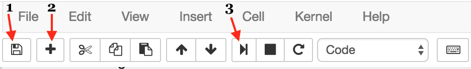
The first button is the button you’ll use to save your work as you go along (1). I won’t give you directions as when you should do this — that’s up to you!
Next, we have the “add cell” button (2). Cells are blocks of code that you can run together. These are the building blocks of jupyter notebook because it provides the option of running code incrementally without having to to run all your code at once.  Throughout this tutorial, you’ll see lines of code blocked off — each one should correspond to a cell.
Lastly, there’s the “run cell” button (3). Jupyter Notebook doesn’t automatically run it your code for you; you have to tell it when by clicking this button. As with add button, once you’ve written each block of code in this tutorial onto your cell, you should then run it to see the output (if any). If any output is expected, note that it will also be shown in this tutorial so you know what to expect. Make sure to run your code as you go along because many blocks of code in this tutorial rely on previous cells.

Preparing the Data

Before we implement our classifier, we need to format the Twitter data. Using sklearn.feature_extraction.text.CountVectorizer, we will convert the tweets to a matrix, or two-dimensional array, of word counts. Ultimately, the classifier will use these vector counts to train.
First, we import all the needed modules:

Next, we must import the data we’ll be working with. Each file is a text file with one tweet per line. We will use the builtin open function to split the file line-by-line and build up two lists: one for tweets and one for their labels. We chose this format so that we can check how accurate the model we build is. To do this, we test the classifier on unlabeled data since feeding in the labels, which you can think of as the “answers”, would be “cheating”. 

Next, we initialize a sckit-learn vector with the CountVectorizer class. Because the data could be in any format, we’ll set lowercase to False and exclude common words such as “the” or “and”. This vectorizer will transform our data into vectors of features. In this case, we use a CountVector, which means that our features are counts of the words that occur in our dataset. Once the CountVectorizer class is initialized, we fit it onto the data above and convert it to an array for easy usage.

As a final step, we’ll split the training data to get an evaluation set through Scikit-learn’s built-in cross_validation function. All we need to do is provide the data and assign a training percentage (in this case, 80%).

Linear Classifier

We can now build the classifier for this dataset. As mentioned before, we’ll be using the LogisticRegression class from Scikit-learn, so we start there:

Once the model is initialized, we have to train it to our specific dataset, so we use Scikit-learn’s fit method to do so. This is where our machine learning classifier actually learns the underlying functions that produce our results.

And finally, we use log_model to label the evaluation set we created earlier:

Accuracy

Now just for our own fun, let’s take a look at some of the classifications our model makes. We’ll choose a random set of tweets from our test data and then call our model on each.

 
Your output may be different, but here’s the random set that my code generated:

Just glancing over the examples above, it’s pretty obvious there are some misclassifications. But we want to do more than just ‘eyeball’ the data, so let’s use Scikit-learn to calculate an accuracy score.

After all, how can we trust a machine learning algorithm if we have no idea how it performs? This is why we left some of the dataset for testing purposes. In Scikit-learn, there is a function called sklearn.metrics.accuracy_score which calculates what percentage of tweets are classified correctly. Using this, we see that this model has an accuracy of about 80%.

The result should be:

0.800498753117

Yikes. 80% is better than randomly guessing, but still pretty low as far as classification accuracy goes. With that said, we just built a classifier with less than 50 lines of Python code and no math. That, my friends, is pretty awesome. Even though we don’t have the best results, sckit-learn has provided us with a solid model, which we can improve on if we tune some of the parameters we saw throughout this post. For example, maybe the model needs more training data? Maybe we should have selected 90% of the data for training instead of 80%? Maybe we should have accounted cleaned the data by checking for misspellings?  

These are all important questions to ask yourself as you utilize powerful machine learning modules like Scikit-learn.

If you liked what you did here, check out my GitHub (@lesley2958) and Twitter (@lesleyclovesyou) for more content!